Synced maps
Two or more maps of the same place, side by side on one extent, read through one cursor — for then-and-now comparisons place by place.
HOLC maps 1935–40 · tracts 2010–15
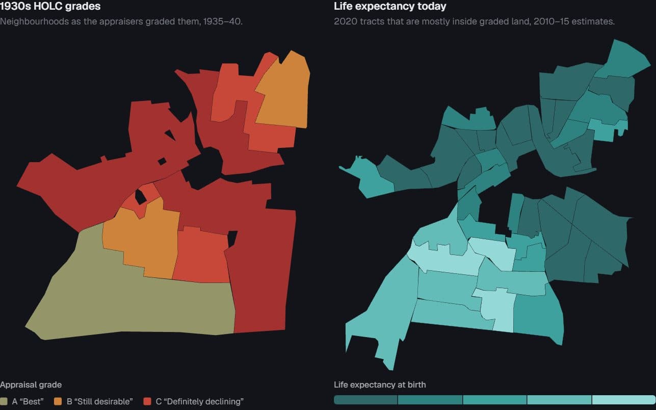
Federal appraisers graded city neighbourhoods A to D in the late 1930s. Beside each 1930s map, the same extent today: census tracts coloured by life expectancy at birth. Point at a place to outline it on both maps.
City
Isolate a grade
In Nashville, people in the 7 tracts graded A now live 82.6 yrs on average; in the 23 tracts graded D, 70.4 yrs — a gap of 12.2 years (population-weighted).
1930s HOLC grades
Neighbourhoods as the appraisers graded them, 1935–40.
Appraisal grade
- A “Best”
- B “Still desirable”
- C “Definitely declining”
- D “Hazardous”
Life expectancy today
2020 tracts that are mostly inside graded land, 2010–15 estimates.
Life expectancy at birth
72768084
ShorterLonger (years)
Point at a 1930s polygon or a 2020 tract: its outline appears on both maps. Tab into a map to step through places with the arrow keys.
The grade is a tendency, not a sentence: every graded tract in the country
Boxes span the middle half of tracts in each grade, whiskers the 5th to 95th percentile, the thick tick the median; dots are the payload's fixed sample of 220 tracts per grade. A tract you point at on the map lands here on its grade's row.
Where the shadow is longest: 29 cities
Tracts graded DTracts graded AD tracts nationwide, 76.8 yrs
How to read the maps. Both panels are fitted to the same extent through one projection, so a place sits at the same spot in each; pointing at either map outlines the same place on both. The left map is the Home Owners' Loan Corporation's security grades as digitized by Mapping Inequality. The right map shows 2020 census tracts that the build assigned a grade because at least half their land lies inside graded polygons; other tracts are not drawn. Each tract takes the grade that covers most of its land. Graded tracts with no life-expectancy estimate were left out of the book's city maps, so they show as gaps rather than as no-data fills.
Measures. Life expectancy at birth is the NCHS small-area estimate (USALEEP) for 2010–15, carried onto 2020 tracts. The income rank is the Opportunity Atlas's mean adult household-income percentile for children raised at the 25th percentile, birth cohorts 1978–83. City gaps compare population-weighted life expectancy in A- and D-assigned tracts, for cities with at least five A and ten D tracts. Gaps here are the difference of the rounded endpoints; the book's published gaps, taken before rounding, differ by 0.1 in five cities (Nashville: 12.3) and are listed in the table. In the dumbbell's tooltip, “Earlier” is the D value and “Later” the A value.
What this cannot show. The appraisers drew red lines around neighbourhoods that were already poorer, more crowded and more often Black, so the gap mixes whatever the maps did with the disadvantage they recorded. Boundary studies find real but smaller causal effects. This is the descriptive ledger, not a causal estimate.
HOLC polygons: Mapping Inequality, University of Richmond Digital Scholarship Lab, CC BY-NC-SA 4.0. Life expectancy: NCHS USALEEP. Mobility: Opportunity Atlas (Chetty, Friedman, Hendren, Jones & Porter). Grades and colours are the appraisers' ranking, reproduced to show what they did.
Nashville tracts · 41 rows
| Tract (GEOID) | 1930s grade | Life expectancy (years) | Adult income rank of children raised poor (percentile) |
|---|---|---|---|
| 47037017701 | A | 79.6 | 47 |
| 47037017800 | A | 80.1 | 45 |
| 47037017901 | A | 81.9 | 43 |
| 47037017902 | A | 82.3 | 58 |
| 47037018500 | A | 83.7 | 47 |
| 47037018000 | A | 84.6 | 47 |
| 47037017702 | A | 84.9 | 50 |
| 47037011400 | B | 71.6 | 30 |
| 47037011700 | B | 73.6 | 31 |
| 47037011200 | B | 74.4 | 33 |
| 47037016800 | B | 79.8 | 46 |
| 47037016700 | B | 83.3 | 43 |
| 47037016900 | B | 84 | 38 |
| 47037011300 | C | 70.8 | 29 |
| 47037016600 | C | 72.9 | 41 |
| 47037017100 | C | 77.8 | 31 |
| 47037012100 | C | 79 | 35 |
| 47037017000 | C | 79 | 35 |
| 47037019300 | D | 66.3 | 27 |
| 47037017200 | D | 67.6 | 37 |
Page 1 of 3
A-vs-D gap by city · 29 rows
| City | A tracts (years) | D tracts (years) | Gap shown (years) | Published gap (years) | A tracts | D tracts |
|---|---|---|---|---|---|---|
| Nashville | 82.6 | 70.4 | 12.2 | 12.3 | 7 | 23 |
| Louisville | 80.5 | 70.5 | 10 | 10 | 6 | 15 |
| Milwaukee Co. | 84.7 | 74.8 | 9.9 | 9.9 | 5 | 37 |
| Indianapolis | 81.1 | 71.3 | 9.8 | 9.8 | 7 | 38 |
| Pittsburgh | 82 | 73.1 | 8.9 | 8.9 | 7 | 33 |
| Cleveland | 80.3 | 72 | 8.3 | 8.3 | 24 | 44 |
| Columbus | 78.9 | 71.5 | 7.4 | 7.4 | 10 | 13 |
| Oakland | 85.2 | 77.8 | 7.4 | 7.4 | 11 | 39 |
| Chicago | 83.3 | 76.5 | 6.8 | 6.8 | 13 | 213 |
| Oklahoma City | 78.1 | 71.2 | 6.9 | 6.8 | 9 | 11 |
| St. Paul | 82.5 | 75.7 | 6.8 | 6.8 | 6 | 12 |
| Des Moines | 79.7 | 73 | 6.7 | 6.7 | 7 | 12 |
| St. Louis | 80.4 | 73.8 | 6.6 | 6.6 | 17 | 15 |
| Miami | 82.4 | 75.9 | 6.5 | 6.5 | 8 | 31 |
| Baltimore | 78.3 | 72.4 | 5.9 | 5.9 | 11 | 37 |
| Essex Co. | 82.3 | 76.6 | 5.7 | 5.7 | 22 | 37 |
| Philadelphia | 79.6 | 73.9 | 5.7 | 5.7 | 27 | 129 |
| San Antonio | 79.9 | 74.2 | 5.7 | 5.7 | 6 | 23 |
| Minneapolis | 81.7 | 76.2 | 5.5 | 5.5 | 8 | 17 |
| Fort Worth | 80.3 | 75 | 5.3 | 5.4 | 5 | 16 |
Page 1 of 2
National tract distribution by grade · 4 rows
| Grade | 5th pct | 25th pct | Median | 75th pct | 95th pct | Tracts | Population-weighted mean |
|---|---|---|---|---|---|---|---|
| A “Best” | 73.5 | 78.3 | 81.1 | 83.4 | 86.5 | 673 | 80.91 |
| B “Still desirable” | 71 | 75.8 | 79 | 81.7 | 85.7 | 2,247 | 79.11 |
| C “Definitely declining” | 69.5 | 74.4 | 77.8 | 80.8 | 84.3 | 5,061 | 77.95 |
| D “Hazardous” | 67.8 | 72.4 | 76 | 79.5 | 83.6 | 2,986 | 76.78 |
Page 1 of 1
Mapping Inequality (University of Richmond DSL); NCHS USALEEP 2010–15; Opportunity Atlas · ZIP Code Destiny, “The Ninety-Year-Old Map”
Preview
How to read it
Point at a place in any panel: it is outlined in every panel and the readout lists what each map says about it. Panels share one projection fit, so a place sits at the same spot in each; compare colours at that spot, not panel against panel.
When to use it
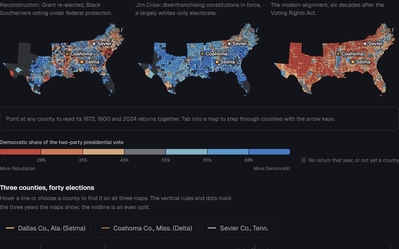
A 1930s map beside the same city today, one county map across several elections, any before-and-after where the question is how each place changed.
Watch out for
Do not fit each panel to its own features — the same place lands in different spots and the comparison is lost. Do not re-range a ramp per panel or per city. Past four panels, use small multiples or a slider.
Data shape & units
Panels: { id, title, features (GeoJSON keyed by feature.id), values: { [id]: number | string | null }, scale }. Scale is { kind: "threshold", breaks, colors } for a quantity or { kind: "ordinal", categories: [{ value, label, color }] } for grades. Panels may share one features array or draw different geometry of the same place; pass extent to make the shared fit explicit.
Missing values
A null or missing value takes the no-data fill and the legend adds a no-data swatch. Places the source dropped cannot be drawn at all — say so in the note; a gap is not a no-data fill.
Controls & accessibility
Hover outlines a place in every panel; click or tap pins it and a second click releases it. Each panel is focusable: arrow keys step through places in id order (alphabetical within each state for US counties), Enter pins, Escape clears. The readout is a live status line and the table carries every value.
Use the component
Install from the CTZN registry, then pass your prepared rows. Examples below illustrate the component contract.
npx shadcn add @ctzn-viz/synced-maps<SyncedMaps projection="albers"
panels={[1872, 1900, 2024].map((y) => ({
id: String(y), title: String(y), features: counties,
values: shares[y], scale: voteScale }))}
mesh={stateBorders}
ariaLabel="County two-party share, 1872, 1900 and 2024" />Examples using this form
US cities · 1930s redlining maps and NCHS tract life expectancy, 2010–15
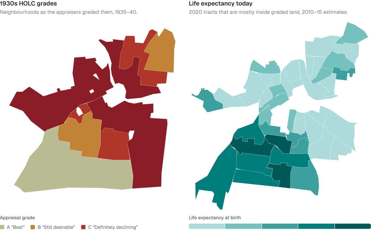
Redlined then, shorter lives now
Do neighbourhoods the 1930s appraisers graded “hazardous” still live shorter lives?
Hides: Cause. Appraisers drew red lines around neighbourhoods that were already poorer and more often Black.
Try it: Switch cities · Point at a place on either map
Eleven former Confederate states · county presidential returns, 1872, 1900, 2024
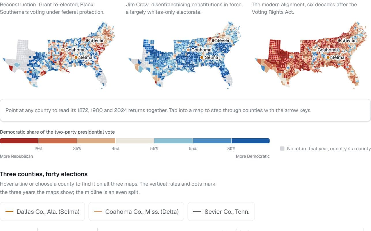
The map remembers, upside down
Does the South’s 1872 county map still predict how its counties vote?
Hides: Who could vote. Jim Crow–era Democratic shares describe a largely whites-only electorate.
Try it: Point at a county