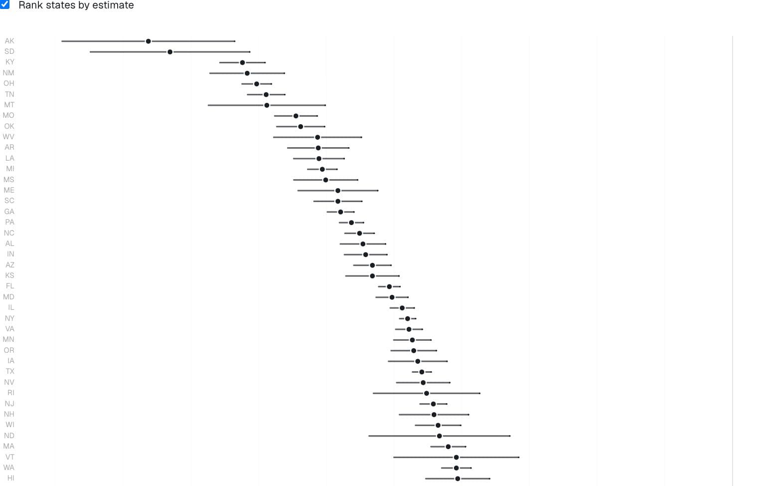
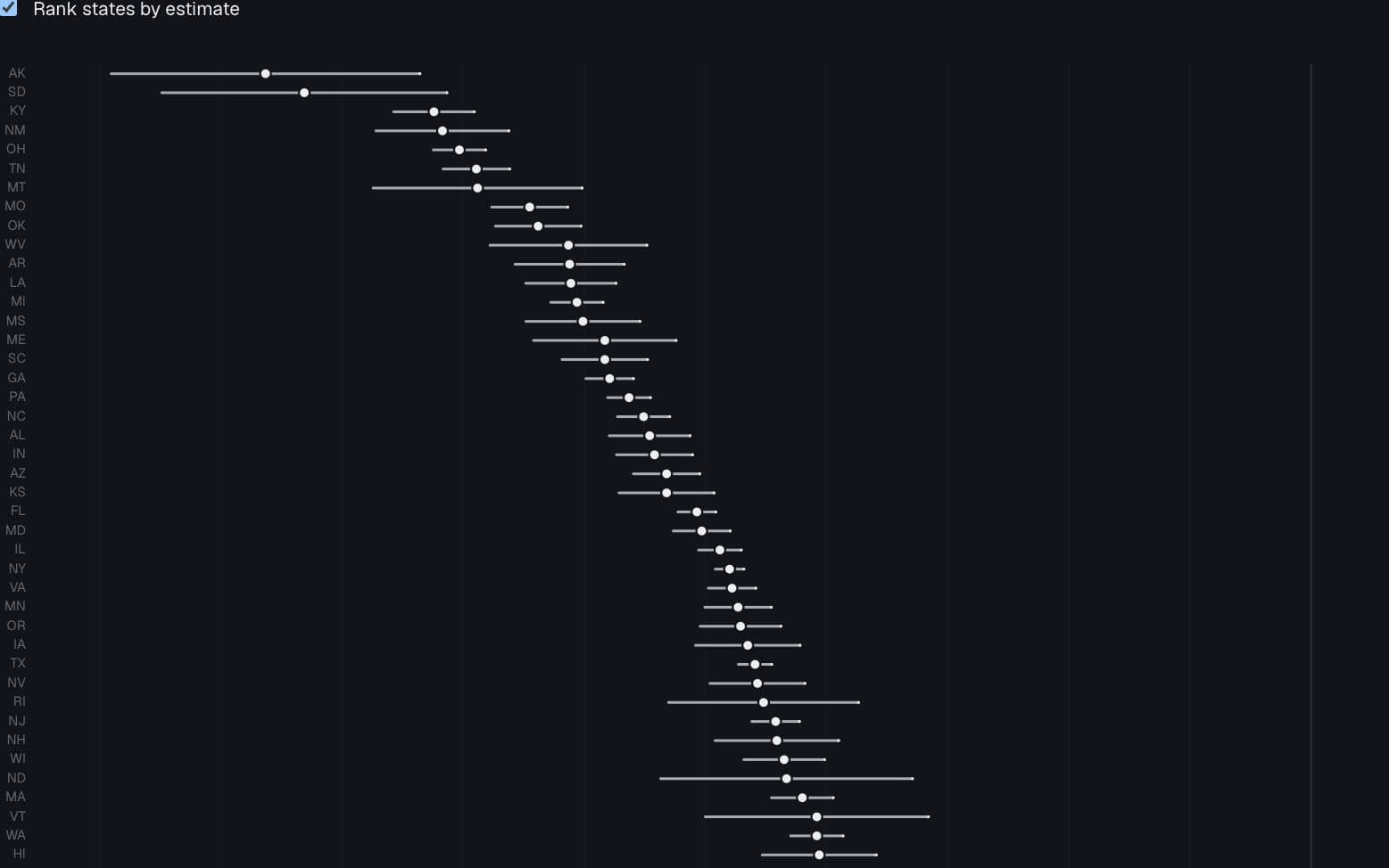
Caterpillar plot
Order a dense set of estimates while retaining their intervals.
Whiskers are approximate normal 95% intervals computed as b ± 1.96 × the supplied standard error. Ranking smooths the visual sequence by construction; it does not establish that neighboring states differ.
Chart data · 49 rows
| Position | State | Estimate (pp) | Lower 95% | Upper 95% |
|---|---|---|---|---|
| 1 | AK | -8.63 | -9.9 | -7.36 |
| 2 | SD | -8.31 | -9.49 | -7.13 |
| 3 | KY | -7.24 | -7.57 | -6.91 |
| 4 | NM | -7.17 | -7.72 | -6.62 |
| 5 | OH | -7.03 | -7.25 | -6.81 |
| 6 | TN | -6.89 | -7.16 | -6.62 |
| 7 | MT | -6.88 | -7.74 | -6.02 |
| 8 | MO | -6.45 | -6.76 | -6.14 |
| 9 | OK | -6.38 | -6.73 | -6.03 |
| 10 | WV | -6.13 | -6.78 | -5.48 |
| 11 | AR | -6.12 | -6.57 | -5.67 |
| 12 | LA | -6.11 | -6.48 | -5.74 |
| 13 | MI | -6.06 | -6.28 | -5.84 |
| 14 | MS | -6.01 | -6.48 | -5.54 |
| 15 | ME | -5.83 | -6.42 | -5.24 |
| 16 | SC | -5.83 | -6.18 | -5.48 |
| 17 | GA | -5.79 | -5.99 | -5.59 |
| 18 | PA | -5.63 | -5.81 | -5.45 |
| 19 | NC | -5.51 | -5.73 | -5.29 |
| 20 | AL | -5.46 | -5.79 | -5.13 |
Page 1 of 3
Captured state income-gradient estimates · tract-income analysis
Preview
How to read it
Each ranked row carries a point estimate and its interval; the reference rule is common to every row.
When to use it
Many comparable state or group estimates with a common estimand.
Watch out for
Switch off sorting: the smooth rising pattern is partly a consequence of rank order. Do not interpret adjacent ranks as statistically distinct.
Data shape & units
{label,estimate,lo,hi}[]; reference defaults to zero. This example derives normal 95% bounds from b ± 1.96 SE.
Missing values
Rows must have finite estimates and bounds; disclose approximate rather than supplied intervals.
Controls & accessibility
Choose an outcome, toggle ordering, and use the table to map positions back to states.
Use the component
Install from the CTZN registry, then pass your prepared rows. Examples below illustrate the component contract.
npx shadcn add @ctzn-viz/forest-plot<ForestPlot data={estimates} sort="ascending" rowHeight={14}
reference={0} ariaLabel="Ranked state gradients" />