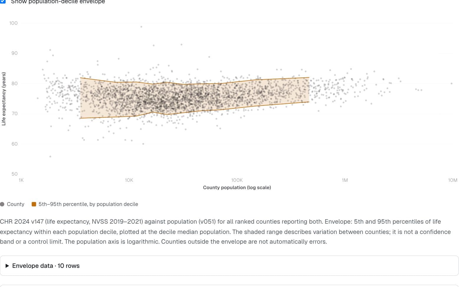
Scatter with empirical envelope
Show how a distribution widens or narrows along another variable.
- County
- 5th–95th percentile, by population decile
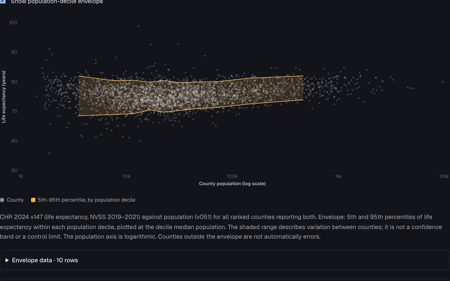
CHR 2024 v147 (life expectancy, NVSS 2019–2021) against population (v051) for all ranked counties reporting both. Envelope: 5th and 95th percentiles of life expectancy within each population decile, plotted at the decile median population. The shaded range describes variation between counties; it is not a confidence band or a control limit. The population axis is logarithmic. Counties outside the envelope are not automatically errors.
Envelope data · 10 rows
| Median population | 5th percentile (years) | 95th percentile (years) | Counties |
|---|---|---|---|
| 3,533 | 68.6 | 82 | 307 |
| 7,513 | 69 | 80.5 | 307 |
| 11,663 | 69.3 | 80.6 | 307 |
| 16,601 | 70.6 | 79.9 | 307 |
| 22,593 | 69.8 | 80.5 | 307 |
| 31,957 | 70.4 | 79.8 | 307 |
| 45,306 | 71 | 80 | 307 |
| 71,403 | 71.4 | 80.1 | 307 |
| 146,140 | 72.6 | 81.3 | 307 |
| 466,103 | 74 | 82.1 | 307 |
Page 1 of 1
County data · 3,070 rows
| County | State | Population | Life expectancy (years) |
|---|---|---|---|
| Autauga County | AL | 59,759 | 75.3 |
| Baldwin County | AL | 246,435 | 76.7 |
| Barbour County | AL | 24,706 | 72.4 |
| Bibb County | AL | 22,005 | 72.3 |
| Blount County | AL | 59,512 | 73.4 |
| Bullock County | AL | 10,202 | 72.1 |
| Butler County | AL | 18,650 | 73.2 |
| Calhoun County | AL | 115,788 | 71.7 |
| Chambers County | AL | 34,088 | 72.5 |
| Cherokee County | AL | 25,302 | 72.7 |
| Chilton County | AL | 45,884 | 73.5 |
| Choctaw County | AL | 12,439 | 73.8 |
| Clarke County | AL | 22,515 | 71 |
| Clay County | AL | 14,198 | 71.8 |
| Cleburne County | AL | 15,346 | 72 |
| Coffee County | AL | 54,805 | 74.2 |
| Colbert County | AL | 58,033 | 73.5 |
| Conecuh County | AL | 11,206 | 69.5 |
| Coosa County | AL | 10,166 | 73.1 |
| Covington County | AL | 37,602 | 71.3 |
Page 1 of 154
County Health Rankings & Roadmaps 2024 · NVSS 2019–2021 life expectancy
Preview
How to read it
Each dot is an observation. The shaded band spans supplied lower and upper percentiles within bins. It describes the distribution, not uncertainty in a fitted mean.
When to use it
Population size versus county outcomes, or any relationship with changing spread and well-defined bins.
Watch out for
Do not call descriptive percentile bands confidence limits or flag every outside point as an error. A log axis needs strictly positive values.
Data shape & units
data: { x, y }[] plus a band overlay { kind: "band", data: { x, lo, hi }[] }. Here x is the median population in a decile, and lo and hi are its 5th and 95th percentiles.
Missing values
Omit invalid observations and incomplete envelope bins. Do not extend the envelope beyond supplied bin positions.
Controls & accessibility
Toggle the envelope to inspect the raw point cloud. Tables expose each county and the ten source percentile bands.
Use the component
Install from the CTZN registry, then pass your prepared rows. Examples below illustrate the component contract.
npx shadcn add @ctzn-viz/scatter-regression<ScatterRegression data={counties} fit="none" logX
overlays={[{ kind: "band", label: "5th–95th percentile", data: deciles }]}
xDomain={[1000, 10000000]} yDomain={[50, 100]}
xLabel="Population (log scale)" yLabel="Life expectancy"
ariaLabel="County life expectancy and population" />